| Introduction |
This report presents the results of a computer simulation analysis performed
by the author as part of TIGHAR’s assessment of Betty’s report
that she heard signals from Amelia Earhart in July 1937, while listening
to her father’s shortwave radio at St. Petersburg, Florida.
This analysis is the product of a team effort. Ric Gillespie, TIGHAR’s Executive Director, relayed
requests to Betty for additional information as the analysis unfolded.
Mike Everette, TIGHAR #2194, provided crucial insights on the design
of Amelia’s transmitter and its tendency to produce harmonic radiation.
And Harry Poole, TIGHAR #2300, researched property records in St. Petersburg,
and took photographs and measurements of Betty’s former house and
adjoining property, thus enabling derivation of the geometry of Betty’s
receiver antenna.
A previous analysis, performed when Betty’s report was received, addressed
the question of whether Betty could have heard Amelia on 3105 kHz (Amelia’s
night frequency) or 6210 kHz (her day frequency). The results showed
that such reception was impossible. The entire propagation path from
Gardner Island to St. Petersburg was in daylight, and the path loss was
too high for reception on either frequency. But Betty’s notebook
was too credible to be dismissed out of hand, so it was decided to consider
alternative explanations. During that process, Mike Everette and the
author concurrently, and independently, recognized the possibility that
Betty heard Amelia on a harmonic of 3105 kHz or 6210 kHz.
Amelia’s transmitter generated the output, or channel, frequency on 3105 kHz
and 6210 kHz by doubling the frequency of an exciter crystal. Hence it
was possible for harmonics of the crystal frequencies to appear in the
output, along with the channel frequency harmonics normally generated
in the transmitter’s final power amplifier. Mike Everette showed
that the design of Amelia’s transmitter output and antenna coupling
circuits did not have any means of harmonic suppression1 and that
consequently, any harmonics present in the transmitter’s output were
passed directly to the antenna and could potentially be radiated.
The question of whether any of those harmonics could propagate a detectable signal
from Gardner Island to St. Petersburg was the starting point for this
analysis.
|
| Methodology |
Computer modeling was used to simulate the propagation conditions for
harmonics that could be produced in Amelia’s transmitter, and to compute
the probability that the signal-to-noise ratio (SNR) required for reception
at Betty’s radio would be available during the period from July
2 through July 9, 1937, between 3 PM and 6 PM, local time in St. Petersburg.
|
| Computer Models |
Two computer models, ICEPAC2 and NEC4WIN95,3 were used in this analysis. Both have been used by the author in previous TIGHAR
signal propagation studies.
ICEPAC was used to simulate the propagation conditions and to calculate the probability
of achieving the required SNR.
NEC4WIN95 was used to derive the frequency-dependent 3-dimensional gain
patterns of Betty’s antenna and Amelia’s antenna (at frequencies above
6210 kHz) for use in ICEPAC, since SNR calculations depend in part upon
the gain of the transmitter and receiver antennas at the respective ends
of the propagation path. The ICEPAC antenna library already included
the gain patterns of Amelia’s antenna at 3105 kHz and 6210 kHz,
derived with NEC4WIN95 for use in previous TIGHAR analyses.
|
| Amelia’s Antenna |
The antenna gain in the direction of St. Petersburg, at harmonic frequencies
up to 15525 kHz, was approximately half the gain at Amelia’s channel
frequencies of 3105 kHz and 6210 kHz. But the gain at harmonics above
15525 kHz was about the same as at the fundamental frequencies. It is
interesting to note that Amelia’s antenna was broadly resonant
between 15.5 MHz to 24 MHz, which would be conducive to radiation of
harmonics in that range.
|
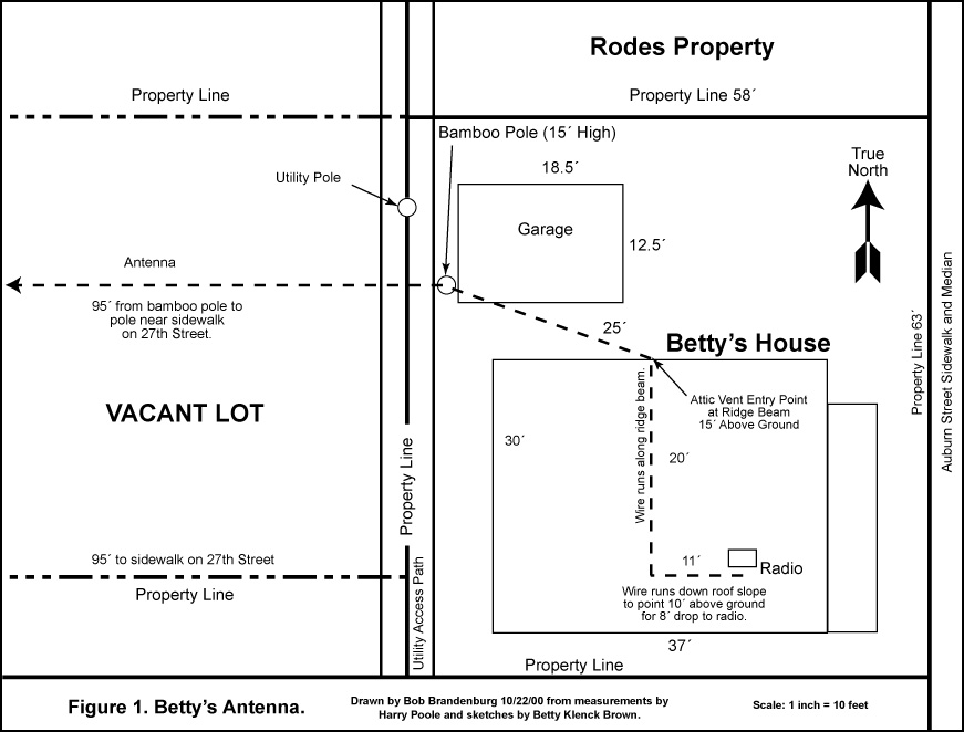
| Betty’s Antenna |
The configuration of Betty’s antenna is shown in Figure
1. The antenna gain
pattern had a broad lobe in the direction of Gardner Island, with a gain
of 2 dB to 3 dB at harmonic frequencies above 12240 kHz. This antenna
had broad resonances at 17 MHz, 23 MHz, and 25 MHz.
|
| Betty’s Radio |
It was important to know the make and model of Betty’s radio, because receiver
sensitivity and tuning range are important factors in evaluating whether
she could have heard signals on a harmonic. Betty did not recall the make and model of her radio, but she provided
information that led to a determination that it probably was a Zenith
model 1000Z “Stratosphere.”4 When shown a color photograph of a Zenith 1000Z that had been restored to new
condition, Betty positively identified it as the model she had used.
The model 1000Z was sold by Zenith during 1935-1938, and was a very capable radio
with extensive shortwave coverage. Approximately 350 sets were produced.
The first 100 production units had shortwave coverage up to 64.3 MHz,
and the remaining sets had coverage up to 45 MHz. The radio had 25 vacuum
tubes, of which 12 were in the audio amplifier section. It had 2 tuned
RF amplifier stages and 2 IF amplifier stages with variable bandwidth.
This radio clearly had the sensitivity and tuning range needed for receiving
signals from Gardner Island.
|
| Required SNR |
The required SNR was set at 3 dB for the purposes of this analysis.
This SNR is half the standard 6 dB level specified5 for just-usable
operator-to-operator communication, and approximates the marginal conditions
described by Betty. She recalls that the signals were “scratchy,”
and that she couldn’t always make out complete phrases. She compares
the quality of the signals to marginal signals heard on a police scanner,
breaking in through the static and then fading out.
|
| The Probability of Achieving the Required SNR |
Signal power and noise power are random variables. Their instantaneous values vary
about their median values, in response to random changes in the propagation
environment. Since the ratio of two random variables is a random variable,
the SNR is a random variable. In an ideal situation, the median SNR is
well above the reception threshold, and the random variations are not
noticed. But in a marginal situation such as described by Betty, the
median SNR is below the reception threshold, and the random variations
occasionally raise the instantaneous SNR above the threshold, permitting
some words and phrases to be recognized.
The probability of achieving the required SNR or better is computed for a specified
percentage of time. The unit of time in this analysis is one hour, and
each hour is uniquely defined in terms of year, month, date, time, radio
frequency, and propagation conditions. For example, if the percentage
of time for the calculation is specified as 5%, then ICEPAC computes
the probability that the required SNR will be achieved in 5% of hours
with identical conditions. Since any given hour occurs once per day,
this is equivalent to the probability that the required SNR will be achieved
on 5% of days with identical conditions at the specified hour.
|
| Identifying Feasible Frequencies
|
Betty does not remember the frequency on which she was listening, but
she does recall that the radio tuning dial pointer was about “an inch or so” to
the right of the top of the dial. That location is in the 18 MHz to 25
MHz region on the dial of a Zenith 1000Z. But that information is not
sufficient for deciding which frequencies should be tested for reception
feasibility.
Feasible frequencies were identified by computing the probability of
achieving the required SNR on all harmonics of the crystal frequencies,
and harmonics of 3105 kHz and 6210 kHz, up to the maximum usable frequency
(approximately 27 MHz) over the propagation path from Gardner Island
to St. Petersburg during the periods of interest. Frequencies with zero
probability of achieving the required SNR were eliminated. In this procedure,
it was assumed that the full rated 50-watt output of Amelia’s transmitter
was delivered to the antenna on each harmonic. Although such harmonic
power levels could not actually be achieved, since harmonic power varies
inversely with the order of the harmonic, this procedure is an effective
method of eliminating infeasible frequencies. If reception was not possible
on a harmonic frequency at 50 watts, then reception on that frequency
would not be possible at any lower power.
This procedure yielded the following feasible frequencies:
| 15525 kHz |
10 x 1552.5 kHz and 5 x 3105 kHz6 |
| 17077.5 kHz |
11 x 1552.5 kHz |
| 18630 kHz |
12 x 1552.5 kHz, 6 x 3105 kHz, and 3 x 6210 kHz |
| 20182.5 kHz |
13 x 1552.5 kHz |
| 21735 kHz |
14 x 1552.5 kHz and 7 x 3105 kHz |
| 23287.5 kHz |
15 x 1552.5 kHz |
| 24840 kHz |
16 x 1552.5 kHz, 8 x 3105 kHz, and 4 x 6210 kHz |
| 26392.5 kHz |
17 x 1552.5 kHz |
The harmonics of 1552.5 kHz (the crystal frequency on the 3105 kHz channel) were
removed from this list to simplify the analysis. The even harmonics were superfluous because
they occur at lower-order (hence higher-power) harmonics of 3105 kHz or 6210 kHz. The odd harmonics would be irrelevant if Betty could have heard Amelia on any harmonic of 3105 kHz
or 6210 kHz. If it turned out that Betty could not have heard Amelia on any harmonic of 3105
kHz or 6210 kHz, then the odd harmonics of 1552.5 kHz could be revisited. As it turned out,
it was not necessary to revisit the odd harmonics.
Removing the harmonics of 1552.5 kHz yielded the following list of feasible frequencies:
| 15525 kHz |
5 x 3105 kHz |
| 18630 kHz |
6 x 3105 kHz and 3 x 6210 kHz |
| 21735 kHz |
7 x 3105 kHz |
| 24840 kHz |
8 x 3105 kHz and 4 x 6210 kHz |
It is not certain that Amelia adhered to her in-flight day/night frequency
plan after arriving at Gardner Island. She could have tried both frequencies,
at every transmission opportunity, in the hope of improving her chances
of being heard. If Amelia transmitted on 3105 kHz, all four frequencies
could be generated as harmonics of 3105 kHz in the transmitter’s
final power amplifier. If she transmitted on 6210 kHz, harmonics at 18630
kHz and 24840 kHz could be generated as in the final power amplifier,
and the even order harmonics of the crystal frequency could be disregarded.
Since Amelia’s actual frequency usage is unknown, all four frequencies
were tested.
It is interesting to note that the final four feasible frequencies generally
agree with Betty’s recollection of where the tuning pointer was
positioned on her radio dial.
|
| SNR Calculations at the Feasible Frequencies |
The probability of achieving the required SNR was computed for each feasible frequency,
for each hour, for specified percentages of days with identical conditions
at each hour, for five harmonic power levels (the 50-watt level used
in the frequency feasibility screening, retained for comparison, and
four reduced power levels).
Terman7 gives the output power level of a well-designed harmonic
generator, as a percentage of output at the fundamental frequency: 2nd
harmonic, 65%; 3rd harmonic, 40%; 4th harmonic, 30%; and 5th harmonic,
25%. The 4 reduced harmonic power levels used in this analysis, and their
respective percentages of 50 watts are: 5 watts (10% ), 1 watt (2% ),
0.5 watt (1%) and 0.1 watt (0.2%). These power levels are conservative
compared to Terman’s values, and are assumed to represent a reasonable
range of harmonic power levels that could be expected at the output of
Amelia’s transmitter.
|
| Results |
The results show that Betty could have heard Amelia on a harmonic.
The probabilities of achieving the required SNR are given in Tables 1 through 5,
and show that hearing Amelia was an unusual, but definitely possible,
event. Table 1 shows the probability that the required SNR would occur
on 1 day out of 20, or 5% of days. Table 2 shows the probability for
2 days out of 20, or 10% of days, and so on. The reader will note that
the probability for a given set of parameters decreases, from table to
table, as the percentage of days increases. This trend indicates that
the conditions required for Betty to hear Amelia were most likely to
occur on 5% of days or less.
The first column in each table shows the date in 1937, the day, and
the sunspot number (SSN), an indicator of ionospheric propagation conditions.
The second column shows the local zone time in St. Petersburg, corresponding
to the time periods described in Betty’s notebook. The third through
sixth columns show the probabilities (in percent) of achieving the required
SNR at each of the four feasible frequencies, in terms of the transmitter
power output to the antenna, in watts. The 50-watt output power level
was retained in the tables to serve as a point of reference for the lower
power levels, and to provide a scaling reference for interpolating the
effects of power levels between 5 watts and 50 watts.
As an example of how to interpret the results, consider the Table 1 entries for
24840 kHz (4 x 6210 kHz) on July 6th during the 1600 hour. For an assumed harmonic power level of 1 watt, there was a
16% probability that the required SNR would occur on 1 day out of 20.
On the next day, the probability is 1%. The sunspot number has increased
from 108 to 143, indicating a higher degree of ionization in the ionosphere,
with correspondingly higher signal absorption losses.
|
| CONCLUSIONS |
- Betty could have heard signals from Amelia at Gardner Island on one
or more harmonics, provided that the power level at the output of Amelia’s
transmitter was 0.1 watt or higher.
- Betty’s recollection of where her radio was tuned, in the general
area of 18 MHz to 25 MHz, is consistent with the frequencies on which
she could have heard Amelia.
- The low probabilities of achieving the required SNR are consistent
Betty’s
description of the fragmentary signals that she heard.
|
| |
| Footnotes |

